Nelson-Seigel 3-factor Model & Forecasting
October 31, 2023 / 5 min read
Last Updated: November 11, 2023In class, we discussed the Nelson-Seigel 3-Factor model of the yield curve. This page estimates the model using daily data from 1/02/2000 to 10/31/2023 for the following maturities of US Treasuries: 3 months, 6 months, 1 year, 2 years, 3 years, 5 years, 10 years, 20 years, and 30 years. The results are then used to forecast the yield curve for November 2023 through an AR(1) model.
1. Data Fetching & Pre-processing
We fetch all the necessary data into a list of lists indexed by maturity dates, then combine into a final processed dataframe.
1library('quantmod')2library(forecast)3library(dplyr)4library(lubridate)5library(YieldCurve)6library(xts)7library(plotly)89# query the data10maturities <- c("DGS3MO", "DGS6MO", "DGS1", "DGS2", "DGS3", "DGS5", "DGS10", "DGS20", "DGS30")11start <- as.Date('2000-01-02')12end <- as.Date('2023-10-31')1314treasuries <- list()1516for (tick in maturities){17# call data18getSymbols(tick, src = 'FRED', from = start, to = end)19treasuries[[tick]] <- get(tick) # R lists can be indexed by name20}21# combine the indexed list to a df22combined_data <- do.call(merge, c(treasuries, all = TRUE))23print(head(combined_data))
2.1 Nelson-Siegel Model
Nelson and Siegel fit the yield at any maturity as follows:
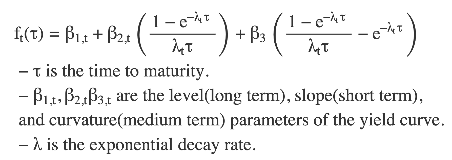
And we can use
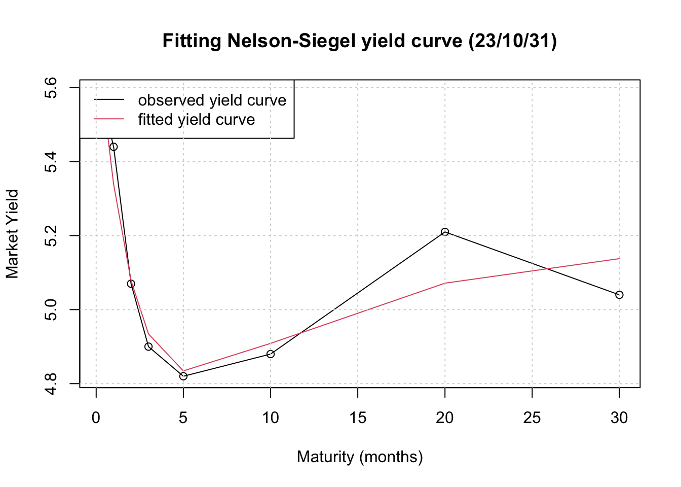
1# NS yield as a function of factors and maturities2# to be used later3calculate_yield <- function(beta_0, beta_1, beta_2, lambda, maturity) {4term1 <- (1 - exp(-lambda * maturity)) / (lambda * maturity)5term2 <- term1 - exp(-lambda * maturity)6yield <- beta_0 + (beta_1 * term1) + (beta_2 * term2)7return(yield)8}910# More cleaning & convert xts to data frame11# make index into a column12combined_data_df <- data.frame(DATE = index(combined_data), coredata(combined_data))13combined_data_df$DATE <- as.Date(combined_data_df$DATE)1415# prepare data for YieldCurve package16yield <- combined_data_df # rename for easier reference17yield$DATE <- as.Date(yield$DATE, format = '%Y-%m-%d')18curve <- xts(yield[, -1], order.by = yield$DATE)19curve_clean <- na.omit(curve) # drop NAs, 5962 obs remaining20maturity.Fed <- c(3/12, 0.5, 1,2,3,5,10, 20, 30 )2122# Nielson-Siegel23NSParameters <- Nelson.Siegel( rate=curve_clean, maturity=maturity.Fed)24y <- NSrates(NSParameters[5962,], maturity.Fed)2526## plotting27plot(maturity.Fed, curve_clean[5962,], main="Fitting Nelson-Siegel yield curve (23/10/31)", xlab=c("Maturity (months)"), ylab=c('Market Yield'), type="o")28lines(maturity.Fed,y, col=2)29legend("topleft", legend=c("observed yield curve","fitted yield curve"),30col=c(1,2),lty=1)31grid()
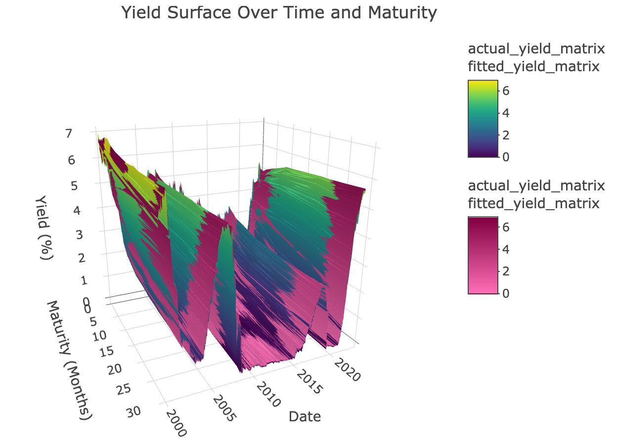
2.2 Nelson-Siegel Fitted & Actual (3D surface)
1# To see our result in 3D, we apply the calculate_yield function to each row in NSParameters2fitted_yield_matrix <- t(apply(NSParameters, 1, function(params) {3sapply(maturity.Fed, calculate_yield, beta_0 = params['beta_0'], beta_1 = params['beta_1'], beta_2 = params['beta_2'], lambda = params['lambda'])4}))56# More cleaning7actual_yield_matrix <- as.matrix(curve_clean)89# Plot the actual yields surface10p <- plot_ly(x = ~rev(maturity.Fed), y = ~yield$DATE, z = ~actual_yield_matrix, type = 'surface',11colorscale = 'Viridis',12name = 'Actual Yields') %>%1314add_surface(x = ~rev(maturity.Fed), y = ~yield$DATE, z = ~fitted_yield_matrix,15colorscale = list(c(0,1),c("rgb(255,112,184)","rgb(128,0,64)")),16name = 'Fitted Yields') %>%17layout(title = "Yield Surface Over Time and Maturity",18scene = list(xaxis = list(title = "Maturity (Months)"),19yaxis = list(title = "Date"),20zaxis = list(title = "Yield (%)")),21width = '70%')2223# Render the plot24p
3.1 Forecasting
Following Diebold & Li (2006), we forecast the yield curve with the following specifications:
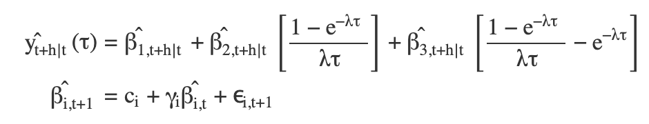
Where we forecast the NS factors (
1# Extract the individual beta factors as separate time series2beta_0_ts <- ts(NSParameters$beta_0, start = c(year(start(NSParameters)), month(start(NSParameters))), frequency = 12)3beta_1_ts <- ts(NSParameters$beta_1, start = c(year(start(NSParameters)), month(start(NSParameters))), frequency = 12)4beta_2_ts <- ts(NSParameters$beta_2, start = c(year(start(NSParameters)), month(start(NSParameters))), frequency = 12)56# Fit AR(1) models to each of the factors7arima_beta_0 <- auto.arima(beta_0_ts)8arima_beta_1 <- auto.arima(beta_1_ts)9arima_beta_2 <- auto.arima(beta_2_ts)1011# Number of days to forecast12forecast_horizon <- length(seq(ymd("2023-11-01"), ymd("2023-11-30"), by = "days"))1314# Forecast the factors for the horizon15forecast_beta_0 <- forecast(arima_beta_0, h = forecast_horizon)16forecast_beta_1 <- forecast(arima_beta_1, h = forecast_horizon)17forecast_beta_2 <- forecast(arima_beta_2, h = forecast_horizon)18lambda <- mean(NSParameters$lambda)1920# For arima_beta_021non_seasonal_order_beta_0 <- arima_beta_0$arma[1:3]22cat("Beta 1 ARIMA(p, d, q):", paste(non_seasonal_order_beta_0, collapse = ", "), "\n")2324# For arima_beta_125non_seasonal_order_beta_1 <- arima_beta_1$arma[1:26273]28cat("Beta 2 ARIMA(p, d, q):", paste(non_seasonal_order_beta_1, collapse = ", "), "\n")2930# For arima_beta_231non_seasonal_order_beta_2 <- arima_beta_2$arma[1:3]32cat("Beta 3 ARIMA(p, d, q):", paste(non_seasonal_order_beta_2, collapse = ", "), "\n")
3.2 Forecasting the yield using the forecasted factors
1# Define the maturities for the yield curve2maturity <- c(3/12, 0.5, 1,2,3,5,10, 20, 30 )34# Initialize a matrix to hold the yield curve forecasts5forecast_dates <- seq.Date(from = as.Date("2023-11-01"), to = as.Date("2023-11-30"), by = "day")6yield_forecasts <- matrix(nrow = forecast_horizon, ncol = length(maturity))78# Calculate the yield curve for each day in Nov9for (i in 1:nrow(yield_forecasts)) {10for (j in 1:ncol(yield_forecasts)) {11yield_forecasts[i, j] <- calculate_yield(12beta_0 = forecast_beta_0$mean[i],13beta_1 = forecast_beta_1$mean[i],14beta_2 = forecast_beta_2$mean[i],15lambda = lambda,16maturity = maturity[j]17)18}19}2021# Combine the forecasted yields with the dates22forecast_df <- data.frame(date = forecast_dates, yield_forecasts)2324# Melt the data frame to a long format for easier plotting and analysis25forecast_df_long <- reshape2::melt(forecast_df, id.vars = 'date', variable.name = 'maturity', value.name = 'yield')
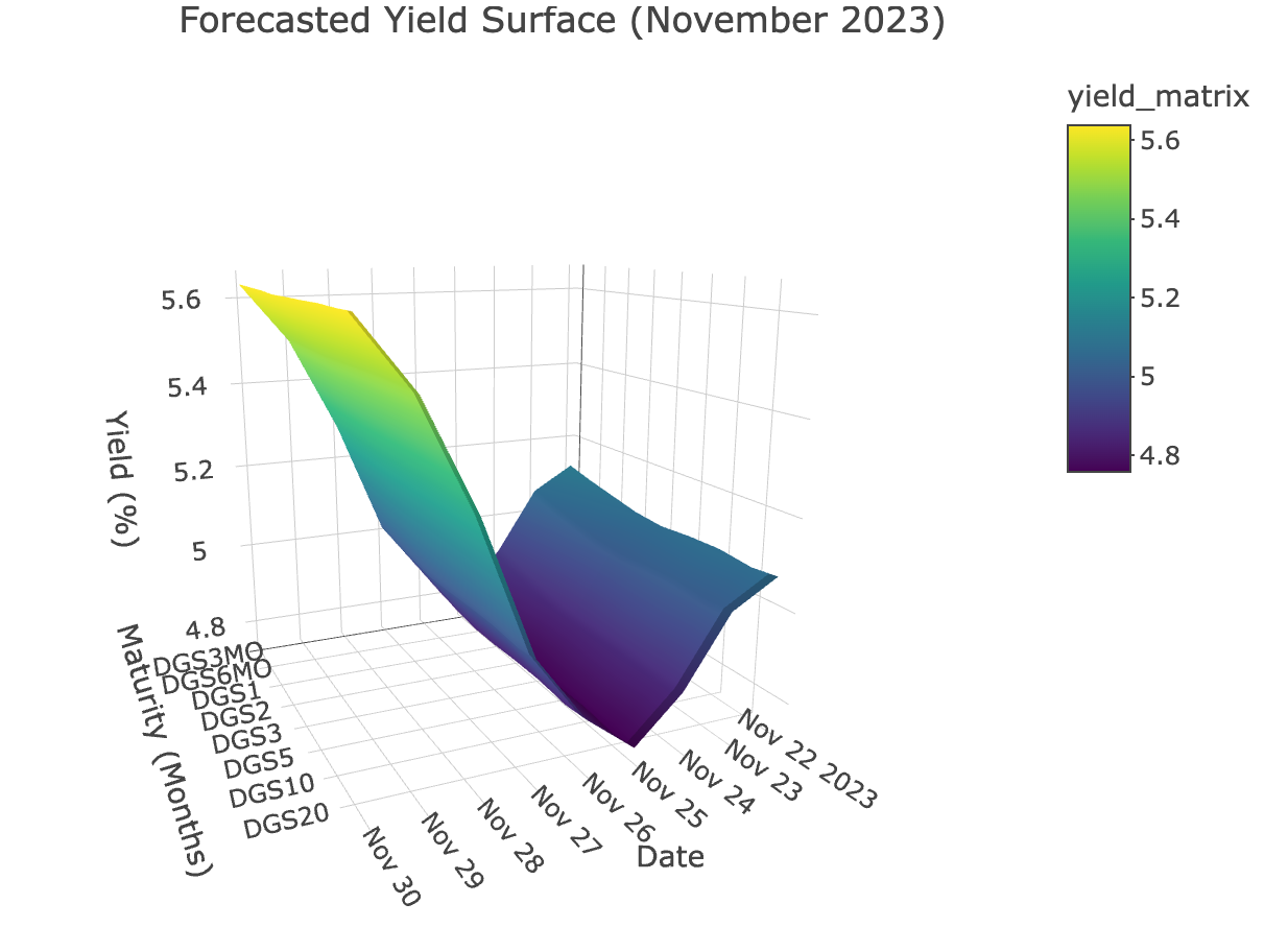
1library(plotly)2yield_matrix <- as.matrix(forecast_df[,-1]) # Excluding the date column34# Use plot_ly to create an interactive 3D plot5plot_ly(z = ~yield_matrix, x = ~rev(forecast_df$date), y = ~maturities, type = "surface") %>%6layout(title = "Forecasted Yield Surface (November 2023)",7scene = list(xaxis = list(title = "Date"),8yaxis = list(title = "Maturity (Months)"),9zaxis = list(title = "Yield (%)")),10width = '70%')
Have a wonderful day.
– Frank
Ready to forecast some yields? Nelson-Seigel is here to help! No stochastic calculus required.